
WCA, Worst-Case Analysis
WCA computes how an electronic function drifts under the combined effects of manufacturing tolerance, temperature, ageing and radiation. The user describes this function as the analytical equations linking its components, and the tool propagates the variability through to every monitored output, returning Begin-of-Life and End-of-Life margins as PPM rejection rates with explicit confidence intervals.
The whole pipeline runs locally on the engineer's workstation. Nothing is sent over the internet, and no data ever leaves the machine.
1 Method ↑
At each Monte Carlo iteration, every component value is drawn from its
statistical distribution and propagated through the user-supplied transfer
function. After N draws (default 10⁶), the
resulting population of output values is compared against the acceptance
interval, and the rejection rate is reported together with its statistical
confidence interval.
Update component database
Import BOM
Define your system equations
Set run parameters
Run & auto-archive
1.1, Sampling distributions
Component models follow datasheet conventions and typical practice in space and defense electronics:
| Component | Variable | Default distribution |
|---|---|---|
| Resistor | R | Uniform on ±tol (BOL); +TC·ΔT and +drift (EOL) |
| Capacitor, X7R / X7S | C | Uniform on ±tol; multiplicative DC-bias derating curve; thermal coefficient; aging shift |
| Capacitor, Tantalum polymer | C, ESR | Uniform ±tol on C; ESR drift law from manufacturer datasheet |
| Inductor | L, DCR | Uniform ±tol; saturation curve from manufacturer datasheet |
| Op-amp | Vos, Ib, GBW, SR | Gaussian truncated to ±3σ on each parameter |
| Voltage reference | Vref, TC | Gaussian on Vref; uniform on TC |
| Diode | VF, IS | Shockley model with temperature-dependent saturation current |
1.2, Confidence interval on rejection rate
Rejection rate is reported with a Clopper-Pearson exact 95% confidence interval. For an observed count of k rejections out of N samples:
p_lo = Beta⁻¹(α/2; k, N − k + 1)
p_hi = Beta⁻¹(1 − α/2; k + 1, N − k)
with α = 0.05. Both bounds are reported in the verdict CSV. The exact form is preferred over the normal approximation because the rejection rate is typically below 1000 PPM, where the Gaussian approximation diverges.
1.3, Extreme quantile estimation (Wilks)
For non-parametric estimation of extreme quantiles without assuming a distribution shape, the framework supports Wilks order statistics. For a target quantile p covered with confidence γ, using the r-th order statistic X(N−r+1) as estimator, the coverage condition is exact:
P( X_(N−r+1) ≥ F⁻¹(p) ) = 1 − I_p(N − r + 1, r) ≥ γ
where Ip(a, b) is the regularized incomplete Beta function (scipy.stats.beta.cdf). Minimum sample size Nmin is solved numerically. Typical values used by the toolchain:
| Order r | p = 99.73% (≈ ±3σ) | p = 99.9% | p = 99.99% |
|---|---|---|---|
| r = 1 (max only) | N ≥ 1 109 | N ≥ 2 994 | N ≥ 29 956 |
| r = 2 | N ≥ 1 572 | N ≥ 4 045 | N ≥ 39 994 |
| r = 3 | N ≥ 1 988 | N ≥ 5 020 | N ≥ 49 419 |
All values for confidence γ = 95%. Higher r trades sample size for robustness against an isolated extreme draw. Default Monte Carlo runs (10⁶) cover all combinations comfortably.
1.4, Sensitivity ranking
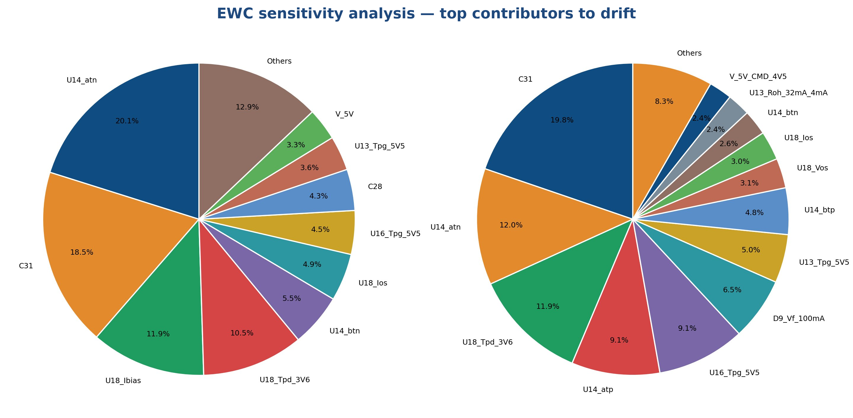
Per-component sensitivity combines a local partial derivative around the
nominal point with the Spearman rank correlation ρ between
sampled inputs and the chosen output. The ranked result is plotted as a
sorted horizontal bar chart. In practice, a small subset of the BOM
accounts for more than 80% of the spread, and that is exactly where the
next design iteration should focus.
1.5, BOL → EOL drift coverage
Each component is sampled across its full drift envelope, from Begin-of-Life to End-of-Life. On top of the manufacturing tolerance, the following contributions are stacked:
| Drift contribution | Modeled as | Typical scale |
|---|---|---|
| Manufacturing tolerance | Uniform on ±tol (datasheet) | 0.1–10% depending on grade |
| Temperature drift | TC × ΔT, additive | −40°C to +125°C junction |
| DC-bias derating (X7R / X7S) | Multiplicative curve, manufacturer datasheet | up to −60% at rated voltage |
| Aging | Logarithmic decay (datasheet) | over mission profile (5–18 years) |
| Radiation (TID) | Lot-tested coefficient, additive | 0 / 25 / 50 krad trajectory |
Radiation drift is fed from actual TID test results when available; otherwise default coefficients from the component database are used and flagged explicitly in the report.
2 Inputs ↑
2.1, Run configuration
Each WCA run is configured through a small set of top-level constants. Component definitions and transfer functions are declared in native Python alongside this configuration:
# ─── Run configuration ─────────────────────────────────────
PPM_THRESHOLD     = 100         # OK/NOK verdict cutoff (PPM)
N_SAMPLES         = 1_000_000   # Monte Carlo sample size
CONFIDENCE_LEVEL  = 0.95        # Clopper-Pearson CI on PPM
WILKS_QUANTILE    = 0.9973      # Wilks target quantile (≈ ±3σ)
WILKS_CONFIDENCE  = 0.95        # Wilks coverage probability
TEMPERATURE_RANGE = (-40, +125) # °C, junction
2.2, Component database
Active components (regulators, op-amps, references, transistors, GaN) are declared in a maintained internal database with all their drift contributions per ECSS-Q-ST-30-11C class. Passive components (resistors, ceramic / tantalum capacitors, inductors) are derived automatically from the BOM, with default drift envelopes pulled from the manufacturer datasheet (TC, DC-bias, aging, TID).
2.3, Optional simulation hooks
For circuits where the transfer function is too complex to write analytically, WCA can call out to an external simulator on each Monte Carlo run:
- Commercial SPICE engines, via batch-mode
.cirnetlist substitution; results parsed from.csvoutput. - LTspice, via
.rawbinary parser (ltspicePython package). - Python-only, closed-form expressions evaluated directly with vectorized numpy operations (~10⁷ samples in seconds).
3 Outputs ↑
Every run produces a deterministic, archivable set of artefacts:
| File | Format | Content |
|---|---|---|
verdict.csv |
UTF-8 CSV | Per-output rejection rate with Clopper-Pearson 95% CI; OK / NOK verdict against the configured PPM threshold |
distrib_*.png |
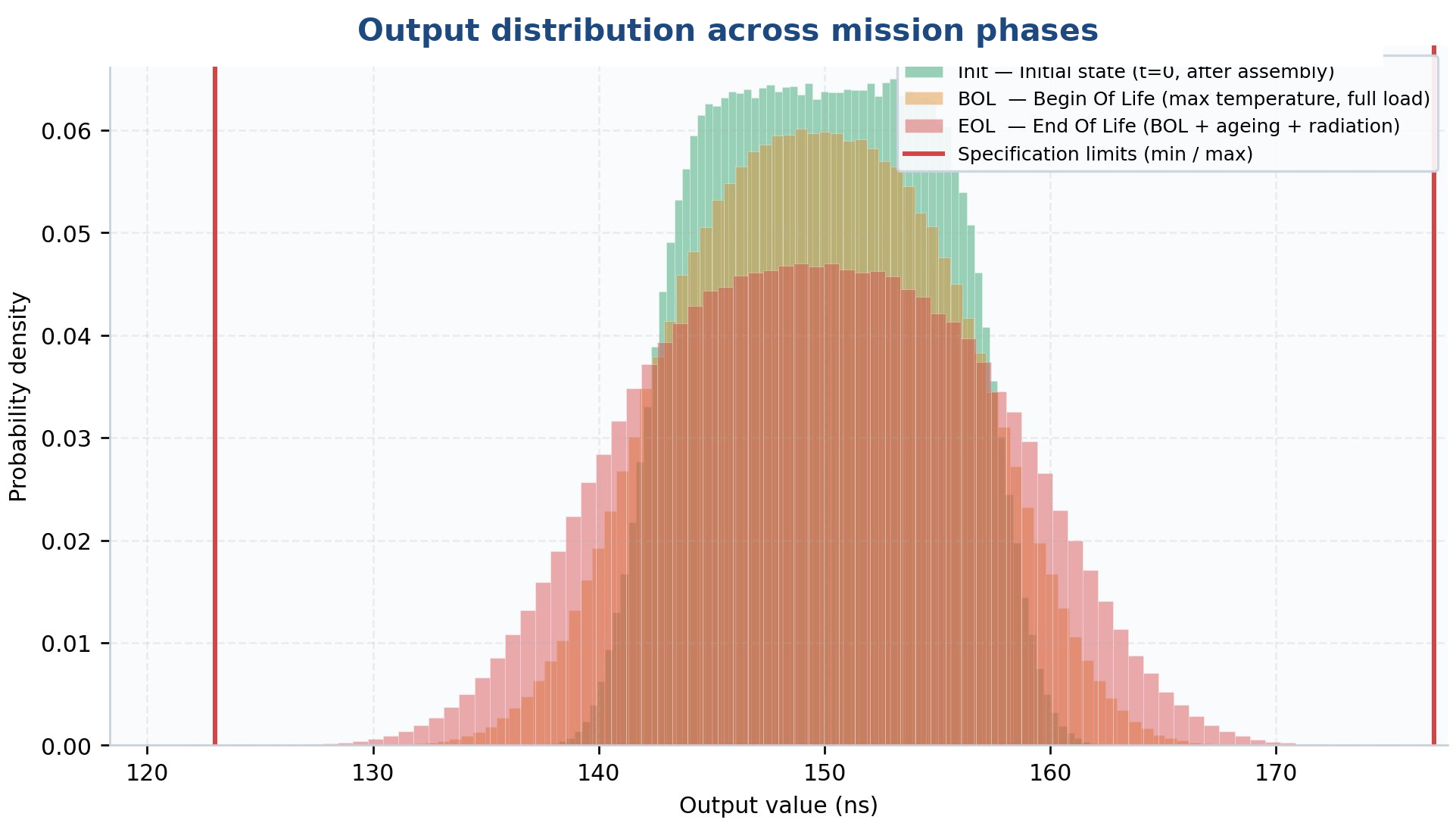
PNG | Histogram of sampled output values with acceptance bounds overlaid; Wilks bins if requested |
sensitivity_*.png |
PNG | Horizontal bar chart of each component's contribution to the output variance, sorted by absolute value |
config.archive.json |
JSON | Full input configuration and seed values for bit-exact reproducibility |
report.docx |
Word | ECSS-formatted report with embedded figures, tables, methodology and version stamp |
All figures follow ECSS chart conventions: labelled axes with units, boxed legend, no chartjunk.
3.1, Sample figures
Three figures produced by every run, illustrating the verdict table, the sensitivity decomposition and the output distribution overlay.

3.2, Reproducibility
Every run archives its random seed, numpy version, and component datasheet revision. Re-running with the archive file produces bit-exact results, even years later, even on a different machine.
4 Standards ↑
| Standard | Scope | Implementation in WCA |
|---|---|---|
| ECSS-Q-ST-30-11C Rev. 2 | Component derating | Per-component derating limits enforced as upper bounds on stress; verdict flags any sample exceeding limits |
| ECSS-Q-ST-60C Rev. 3 | EEE component selection | Used for class assignment and EOL drift assumptions per quality level |
| ESCC-25500 | Diode characterization for space | Shockley model parameters extracted from ESCC-compliant datasheets |
| MIL-HDBK-217F | Reliability prediction (informative) | Optional, failure-rate cross-check on critical components |
| IPC-2221 | PCB design rules (informative) | Used as input bound when WCA is run jointly with thermal models |
4.1, Class mapping
Component derating limits are loaded from a class-indexed table (Class 1 / Class 2 / Class 3 per ECSS-Q-ST-60C). The class is set per run; switching from Class 3 (deep-space) to Class 1 (terrestrial) only requires changing one configuration field, the toolchain re-runs unchanged.
5 Limitations ↑
WCA is an analytical tool. It complements physical characterization but does not replace it. Honest limitations:
- Distribution assumptions. Default distributions, uniform on tolerance and truncated Gaussian on op-amp parameters, reflect typical practice but are not verified for any specific production lot. Lot-specific characterisation is recommended for Class 1 missions.
- Component coupling. Components are sampled independently by default. Correlated drift, for example a matched resistor pair on the same die, has to be modelled explicitly via shared random variables. The framework supports this, but the coupling has to be declared manually.
- Sample size vs computation time. 10⁶ runs are typical; 10⁷ has been tested and takes about 2 minutes per Monte Carlo on a standard workstation. Below 10⁵ runs, the Clopper-Pearson interval widens noticeably, and PPM verdicts become unreliable.
- Simulator coupling overhead. When an external SPICE simulator is invoked at each Monte Carlo iteration, throughput drops to about 1 000 runs per minute. For runs above 10⁵, batch substitution is required.